Assignment 6 - Dissimilarity Index and Multiple Regression

Part I – Dissimilarity Index

White compared to Black:

∑ |a-b| = 90.56

DI = 45.28 – meaning 45.28% of black people would have to move in order to have an equal distribution of white people and black people.

White compared to Asian:

∑ |a-b| = 78.93

DI = 39.46 – meaning 39.46% of Asians would have to move in order to have an equal distribution of white people and Asians.

White compared to Hispanic:

∑ |a-b| = 77.45

DI = 38.73 – meaning 45.28% of Hispanics would have to move in order to have an equal distribution of white people and Hispanics.

Map of Dune County with the percentage of minorities by census tract.

These results show that around 40% of the population would have to move in order to have an even distribution of the races in each census tract. The maps show that Non-Whites are by far concentrated in the central parts of Madison and Dane County. Non-whites would have to move out into the suburbs of Madison and the surround small towns in Dane County in order to have an equal distribution of Whites and Non-whites.

Part II – Kitchen Sink

 

SPSS results of a Kitchen Sink Approach.

Hypotheses

The Null Hypothesis is that there is no linear relationship between Number of Foreclosures per 100 persons and High Cost Loans. The Alternative Hypothesis is that there is a linear relationship between Number of Foreclosures per 100 persons and High Cost Loans.

The Null Hypothesis is that there is no linear relationship between Number of Foreclosures per 100 persons and Percent of people with Mortgages. The Alternative Hypothesis is that there is a linear relationship between Number of Foreclosures per 100 persons and Percent of people with Mortgages.

The Null Hypothesis is that there is no linear relationship between Number of Foreclosures per 100 persons and Percent of Black people. The Alternative Hypothesis is that there is a linear relationship between Number of Foreclosures per 100 persons and Percent of Black people.

The Null Hypothesis is that there is no linear relationship between Number of Foreclosures per 100 persons and Percent of White people. The Alternative Hypothesis is that there is a linear relationship between Number of Foreclosures per 100 persons and Percent of White people.

The Null Hypothesis is that there is no linear relationship between Number of Foreclosures per 100 persons and Percent of Non-white people. The Alternative Hypothesis is that there is a linear relationship between Number of Foreclosures per 100 persons and Percent of Non-white people.

The Null Hypothesis is that there is no linear relationship between Number of Foreclosures per 100 persons and Percent of Asian people. The Alternative Hypothesis is that there is a linear relationship between Number of Foreclosures per 100 persons and Percent of Asian people.

The Null Hypothesis is that there is no linear relationship between Number of Foreclosures per 100 persons and Unemployment. The Alternative Hypothesis is that there is a linear relationship between Number of Foreclosures per 100 persons and Unemployment.

The Null Hypothesis is that there is no linear relationship between Number of Foreclosures per 100 persons and Commuting Minutes. The Alternative Hypothesis is that there is a linear relationship between Number of Foreclosures per 100 persons and Commuting Minutes.

The most significant variables were HighCostLoans and PerMortgage10. I know this because of their low significance values which were close to 0; no other variables had significance values under the required 0.05. They also had positive betas which show that they increase as the dependent variable increase.

At first there was some multicollinearity because of the variable PerBlack. I knew this because of the Eigen value that were close to zero and the condition indexes that were over 30. Once I had removed this variable the multicollinearity disappeared.

PerNonwhite was exclude right away meaning that the variable was just so far from significant the regression didn’t include it. I then removed the remaining variables that were not found significant which included PerWhite, ComMins10 and Unemploy10, PerAsian. I had to rerun the statistics five times in order to get my final equation by removing the least significant variable each time until there were only significant variables left.

At first the significance value was 0.090 for PerMortgage10 but by the time that I had eliminated all other variables beside PerMortgage10 and HighCostLoans the significance value had gone down to 0.017 which is below the 0.05 needed to be significant.

For Number of Foreclosures per 100 persons and High Cost Loans I reject the null hypothesis. There is a linear relationship between the two.

For Number of Foreclosures per 100 persons and Percentage of people with mortgages I reject the null hypothesis. There is a linear relationship between the two.

For Number of Foreclosures per 100 persons and Percent of Black people I fail to reject the null hypothesis. There is no linear relationship between the two.

For Number of Foreclosures per 100 persons and Percent of White people I fail to reject the null hypothesis. There is no linear relationship between the two.

For Number of Foreclosures per 100 persons and Percent of Non-white people I fail to reject the null hypothesis. There is no linear relationship between the two.

For Number of Foreclosures per 100 persons and Percent of Asian people I fail to reject the null hypothesis. There is no linear relationship between the two.

For Number of Foreclosures per 100 persons and Unemployment I fail to reject the null hypothesis. There is no linear relationship between the two.

For Number of Foreclosures per 100 persons and Commuting Minutes I fail to reject the null hypothesis. There is no linear relationship between the two.

My final equation is y = -0.10 + 0.004x₁ + 0.004x₂

The variables are

y = Number of Foreclosures per 100 persons (Count2011)

x₁ = High Cost Loans (HighCostLoans)

x₂ = Percent of people with mortgages (PerMortgage10)

My results show that high cost loans and percent of people with mortgages have significant correlations with the number of foreclosures per 100 persons. I can use this equation to predict the number of foreclosures per 100 persons in a given census tract if I have the data for high cost loans and percent of people with mortgages.

Part III – Stepwise

SPSS results from a Stepwise Regression.

I ended up with the same model as the Kitchen Sink Approach:

Final equation is y = -0.10 + 0.004x₁ + 0.004x₂

The variables are

y = Number of Foreclosures per 100 persons (Count2011)

x₁ = High Cost Loans (HighCostLoans)

x₂ = Percent of people with mortgages (PerMortgage10)

The Stepwise Regression gives me the same model and equation as the Kitchen Sink Approach, however it does it in one step instead of multiple. That’s awesome that the stepwise approach can do all of that analysis by itself; it saves time in having to rerun the regression over and over until I get an equation.

Prediction:

x₁ = 80.0 High Cost Loans

x₂ = 50.0% Drive to Work

y = -0.10 + 0.004(80.0) + 0.004(50.0)

y = -0.10 + 0.32 + 0.20

y = 0.42

According to my model, having 80 high cost loans and 50% of people driving to work in a given census tract you will get 0.42 foreclosures per 100 persons in that census tract.

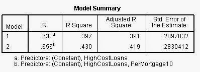
I am somewhat confident in my results due to the okay R² value of 0.430 that I had in my model. The high significance that the two variables I used helps the confidence that I have in the model, but the R² value is the most important sign of the strength of a model. So, I would say that my model is moderately adequate.